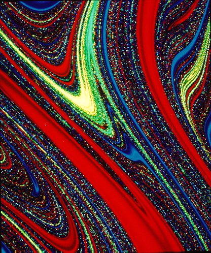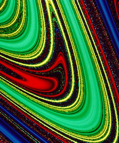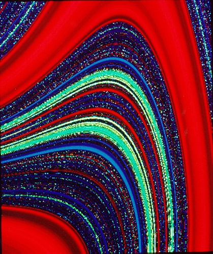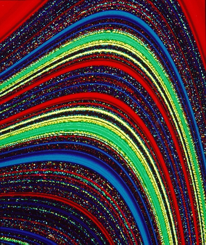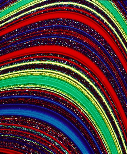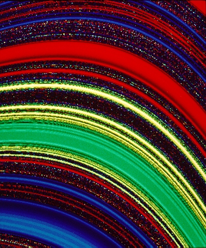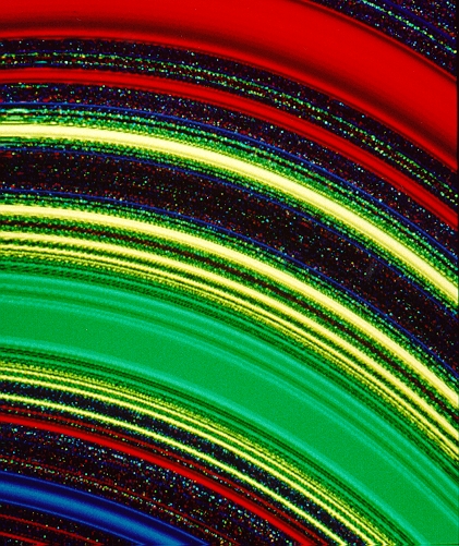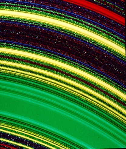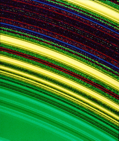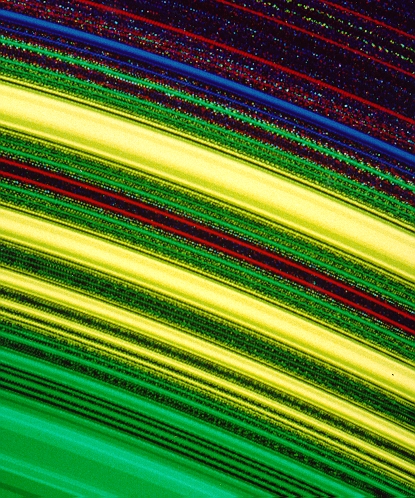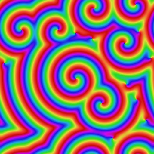
Chaotic Scattering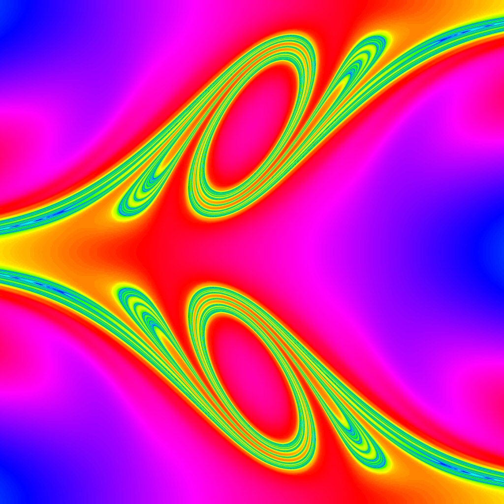
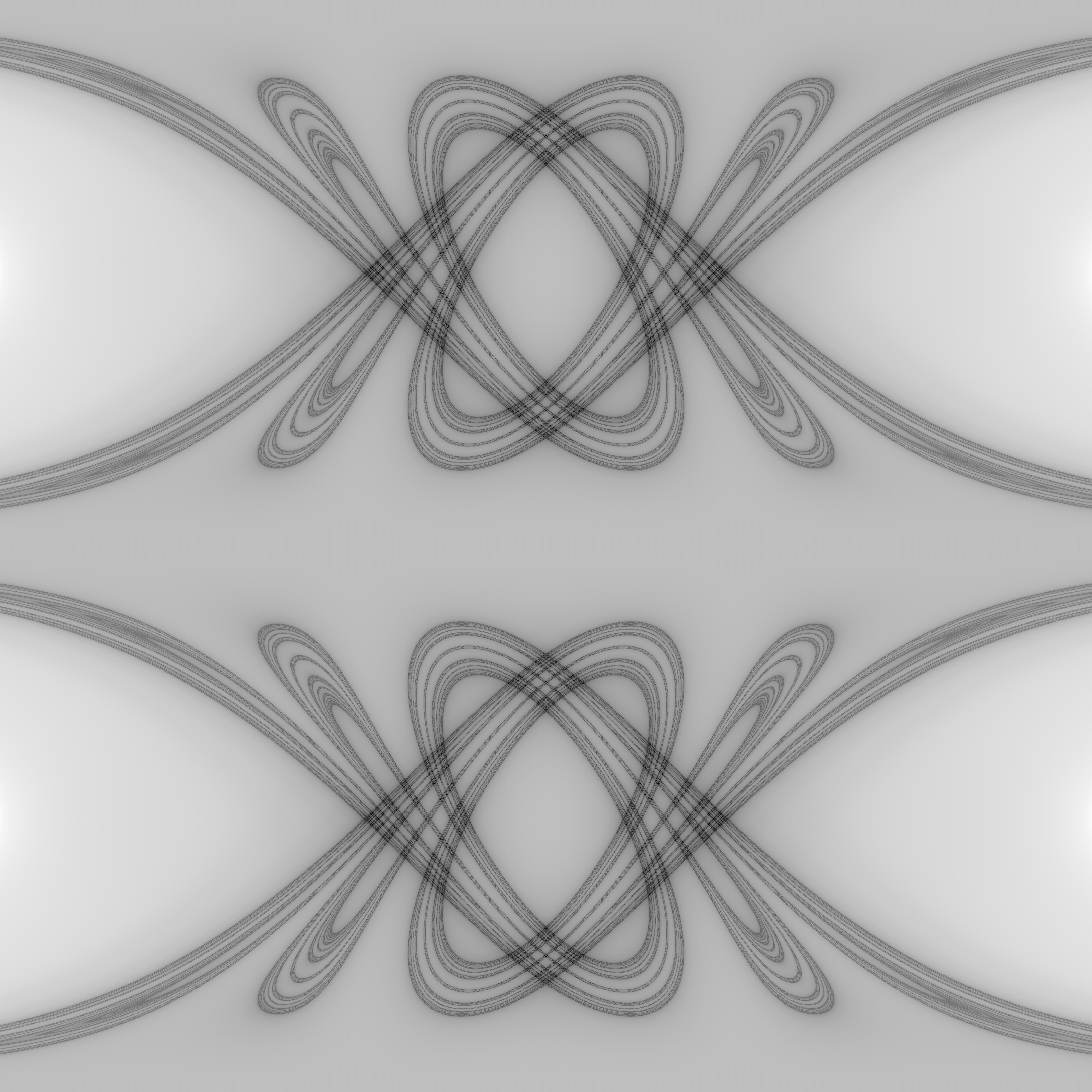
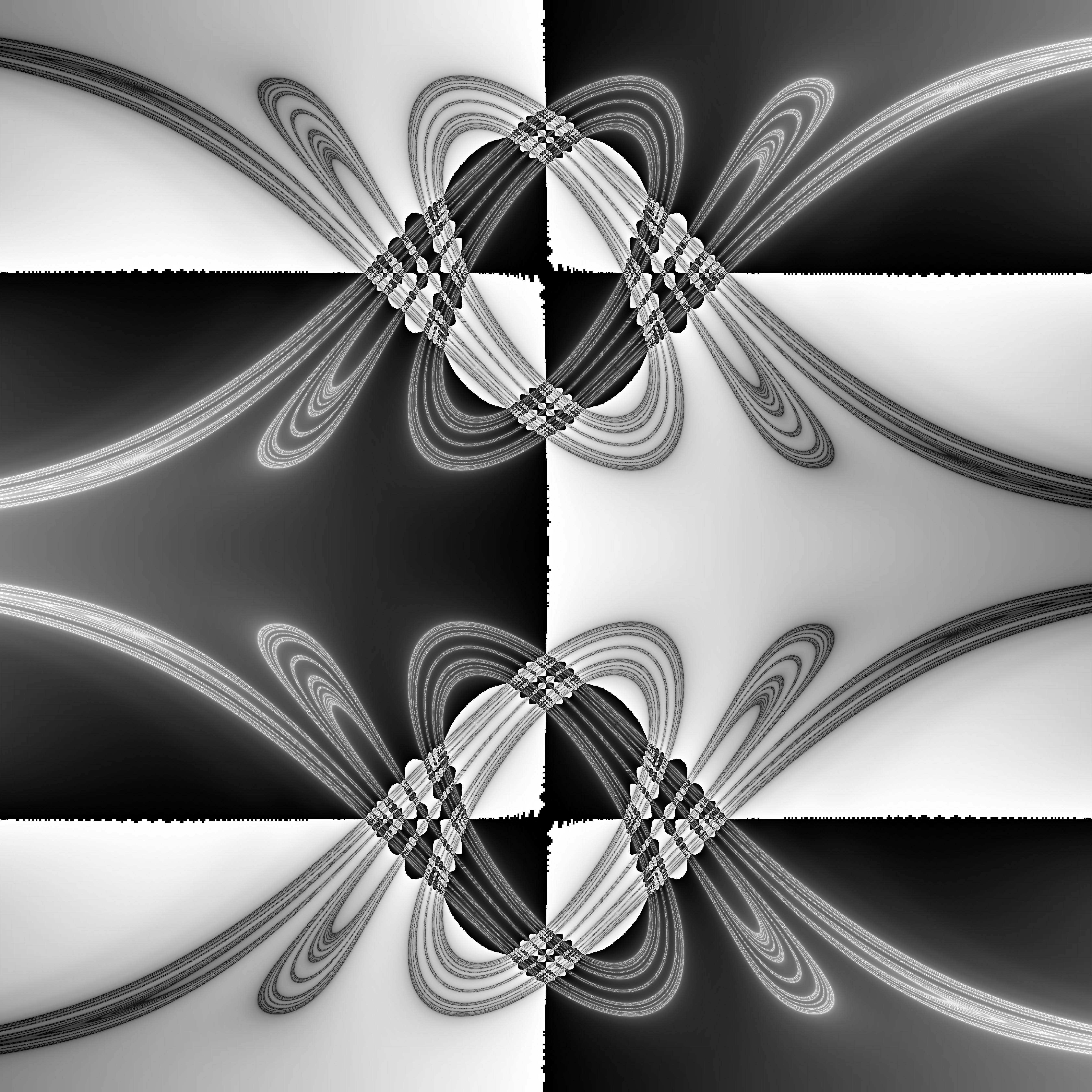
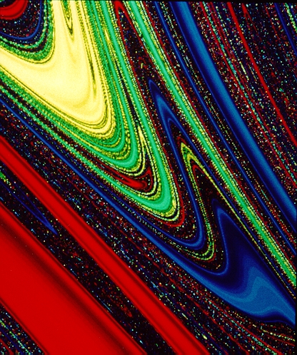
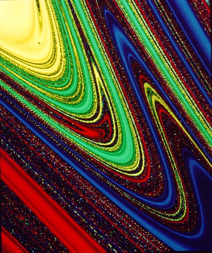
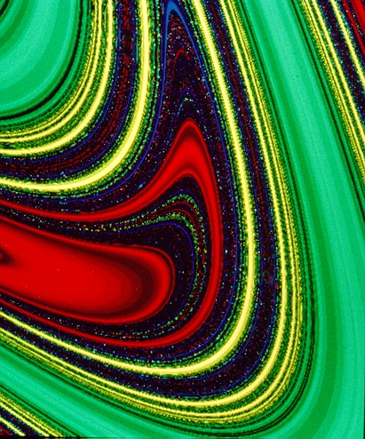
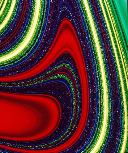
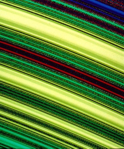
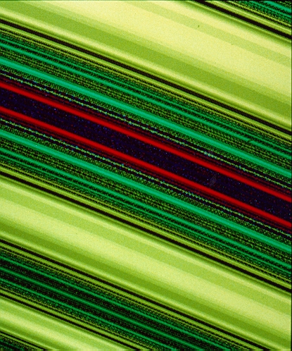
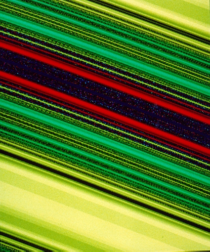
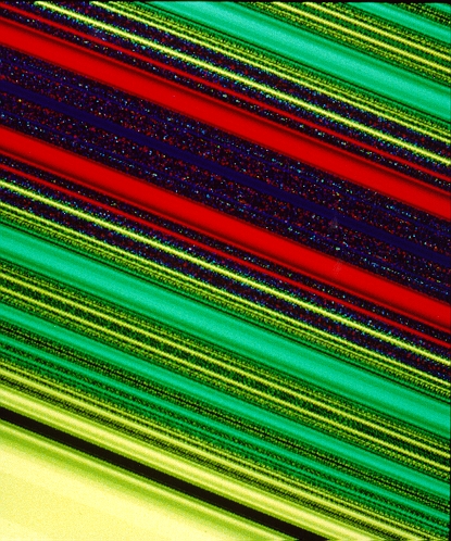
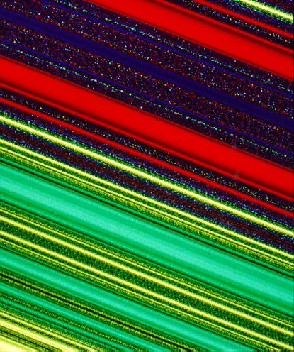
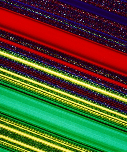
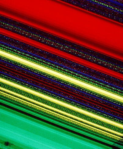
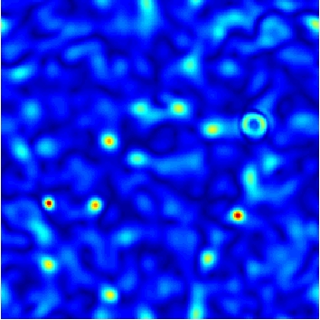
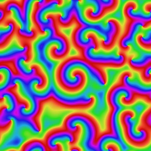
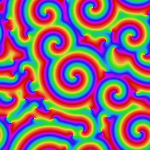
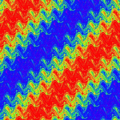
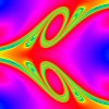
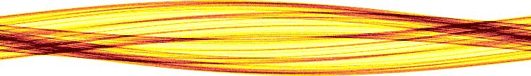
Description: Plot of a cross section of the stable manifold of the chaotic invariant set from scattering off a potential of the form V(x,y)=(x^2)*(y^2)*exp[-(x^2+y^2)]. Created by taking a grid of initial conditions (initial x coordinate,initial velocity angle theta) at a given energy and integrating them forward. The color is proportional to the time the particle remains trapped. The stable manifold appears smooth and swirling along one direction with fractal structure transverse to that direction. The intersection of the stable and unstable manifolds is the nonattracting chaotic invariant set itself (for more details, see Edward Ott's book, "Chaos in Dynamical Systems", Second Edition, 2002). The second graphic is an illustration of this set, and the third is the same with an interesting background.
Attractor PicturesIkeda AttractorThe pictures below show the strange attractor that results from the time evolution of an optical cavity containing a nonlinear dielectric subjected to a periodic string of light pulses. The picure is a cumulative plot of the phase
KAM islandsThis is probably a picture of the Standard map which is a Hamiltonian (conservative) system. An obvious feature of the picture is the KAM islands.
Tinkerbell AttractorThe Tinkerbell attractor is represented by the curve and its basin of attraction is represented by the black color. Other colors denote points which escape to infinity as one continually iterates the two-dimensional map. The colors are shaded according to how fast the points escapes to infinity.
Basin PicturesForced Damped Pendulum...with Four BasinsEven something as simple as a periodically forced damped pendulum can have complex behavior. The computer-generated images below show initial positions that asymptote to one of different behaviors (one color for each behavior). For example, orbits starting at points in the blue region would yield a different type of motion from orbits starting in the red region. The brighter the shade of color, the longer it takes to settle into the corresponding motion. The different regions are separated by fractal basin boundaries. The pictures are made at increasing magnification levels.
...with Two Basins
Fractal FoamThere are three simple attractors (straight lines in fact!) which formed sort of a triangle; however, the basins of attraction is anything but simple. These pictures are the starting points for the interesting ideas of riddled basins.
Wada BasinsWhile many chaotic systems possess boundaries separating basins that are typically fractal, they may also possess the stronger property that any point which is on the boundary of one basin is also simultaneously on the boundary of all the other basins. This interesting property is known as the Wada property. Wada boundaries are to be contrasted with more usual boundaries such as those on a map showing the countries of Europe: there is only a finite number of boundary points that are on the boundary of more than two countries. A simple system exhibiting this interesting Wada property is the three-disk model studied extensively in the context of chaotic scattering. For more information about Wada basin boundaries in this system, check out the paper "Wada Basin Boundaries in Chaotic Scattering."
Coherent StructureThis is not exactly a basin picture, but I didn't feel like creating a new page just for this one picture. However, this is still a special picture for me as it is my first published chaos artwork! For details, check out the paper "Controlling Complexity."
Simulations and ExperimentsDescription: A model of Earth's core, basically a spherical annulus of liquid sodium between a solid inner sphere (20 cm diameter) and a spherical outer container (60 cm). We can independently drive the two spheres to rotate, and we can apply dc external magnetic fields with a pair of magnets. Lately we've been studying inertial waves (a long-known phenomenon in rotating fluids) in the apparatus. What we actually measure is the oscillating magnetic field induced by the presence of the waves. Though the induction itself is linear, the excitation and amplification of the waves is not, and probably depends on instabilities. We've been able to show that the induction patterns are consistent with the induction due to specific (known) inertial wave velocity fields in a sphere. A spectrogram of the signal coming from one of our probes. For this data, the outer sphere is held at 30 Hz and the inner sphere rotation rate is varying along the horizontal axis. The vertical axis is signal frequency, and the color indicates spectral power at that frequency. Red areas have about 100x more power than blue. 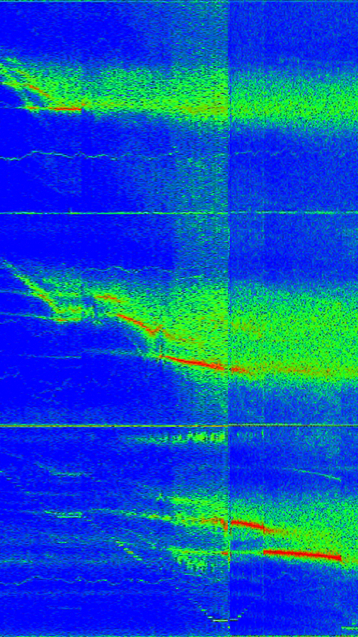
A plot of the measured magnetic field of one of our wave modes. We're measuring the component of the field along a cylindrical radius (i.e., pointing outward from the axis of rotation) over the whole sphere. Theta and phi are the polar and azimuthal coordinate, respectively. 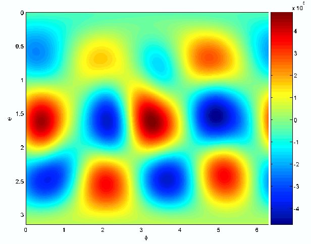
Theoretical calculation of the velocity and kinetic energy fields of the inertial wave mode that we believe is producing the induction shown in the second figure. 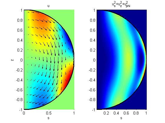
Demonstration of the sensitive dependance on initial conditions in a Rayleigh-Benard convection simulation. The fluid is in a state of spiral defect chaos. Plotted is the difference between two perturbed initial conditions. 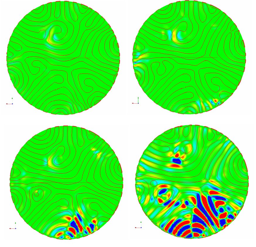
A vector field of the mean flow in a Rayleigh-Benard convection simulation. The collors indicate regions of hot (red) and cold (blue) fluid. 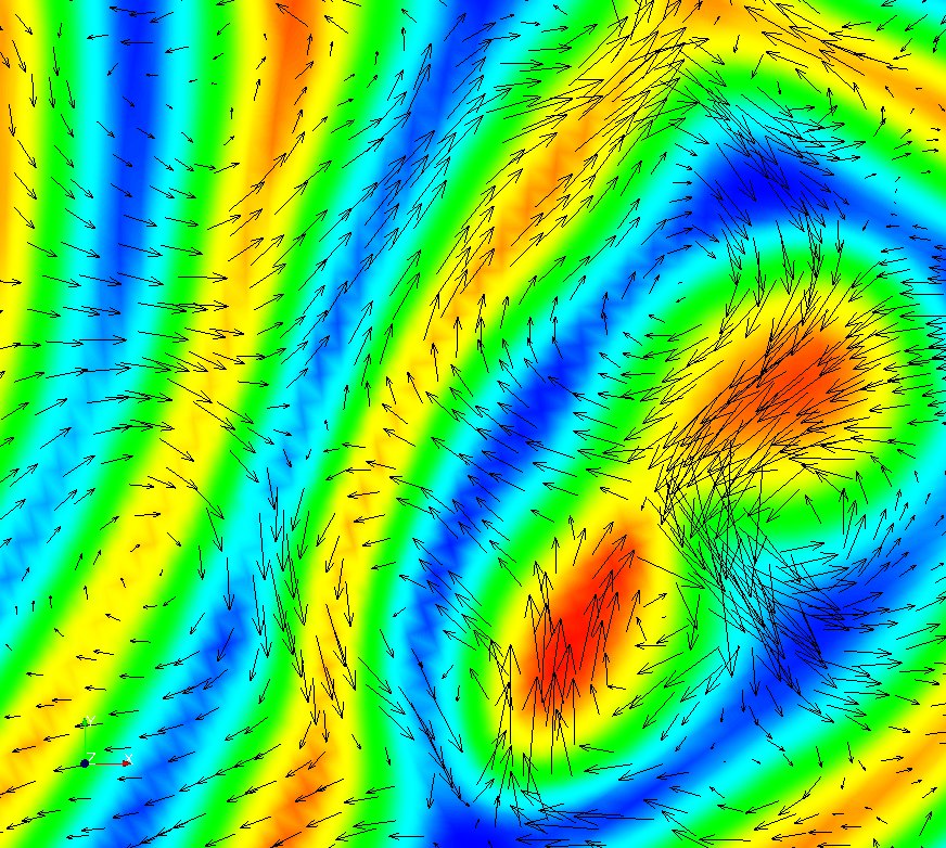
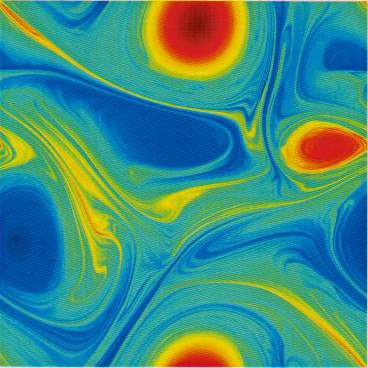
Pattern FormationChaotic Advection of Passive ScalarThe distribution of dye in a fluid undergoing chaotic motion evolves in such a way that the gradient of the dye density increases with time and the region where the dye density gradient is largest becomes more and more striated into thinner and thinner ribbon-like regions, eventually concentrating on a fractal set. These pictures show the early stage of this process.Reference: F. Varosi, T.M. Antonsen and E. Ott, "The spectrum of fractal dimensions of passive scalar gradients in chaotic fluid flows", Phys. Fluids A, vol. 3, p.1017 (1991) Two Dimensional Turbulence
[K. Nam, et al., Phys. Rev. Lett., 84, 5134(2000)] (PDF)
|